The question this post answers

If you’re running an IVF-based vector index over hundreds of millions of CLIP embeddings, two knobs decide your cost and your recall:

• nlist — how many clusters you partition the corpus into.
• nprobe — how many of those clusters you actually search at query time.

The common advice is “set nlist ≈ √N and pick nprobe by taste.” That’s fine for a 1M-vector toy. At 100M–1B+ it stops being useful — the recall-vs-bytes-scanned curve has sharp diminishing returns, and where you sit on that curve is the difference between a $200/mo and a $20,000/mo bill.

This post is the result of building a real calibration workflow on two open datasets, and what the numbers actually look like.

---

The two datasets

Dataset	Embedding	Dim	Vector count	On-disk size (float16)
LAION-400M	CLIP ViT-B/32	512	~407M (410 shards × ~1M)	~410 GB
DataComp-1B	CLIP ViT-L/14	768	~1.4B (1880 shards × ~1M)	~2.3 TB

Both are stored as .npy shards on HuggingFace. LAION-400M fits on a single 1 TB local NVMe; DataComp-1B does not — its scaling sweep streams shards on demand from HuggingFace on a RunPod box.

Why CLIP

CLIP image embeddings are the canonical “big public dataset that looks like a real production workload”: they’re high-dim, dense, not toy-clean, and someone else paid to compute them. ViT-B/32 (512-dim) is the smaller, more common variant; ViT-L/14 (768-dim) is the heavier one used by DataComp. The recall numbers in this post are entirely in image-embedding L2 space — if your workload is text or hybrid, the relative shape of the curves will hold but the absolute numbers will shift.

---

SPANN, SPFresh, and Weaviate’s implementation

SPANN (Microsoft, NeurIPS 2021) is the design pattern this post is implicitly testing. The idea:

• Cluster the corpus into nlist posting lists with k-means.
• Keep only the centroids in RAM — small, ~nlist × dim × 4 bytes.
• Posting lists live on disk (or S3): each list is the actual vectors that landed in that cluster.
• At query time: rank centroids → fetch the nprobe closest posting lists from storage → brute-force scan those vectors → merge top-k.

This is the only design that scales to billions of vectors without billions of GB of RAM. Everything that follows in this post is a SPANN-style calibration.

SPFresh (Microsoft, SOSP 2023) extends SPANN with online updates via the LIRE protocol — incremental insertions and deletions without rebuilding the whole index. That’s the property you want for a live production system.

Weaviate’s HFresh index (technical preview, released in v1.36 on March 3, 2026) is the most production-ready SPFresh-inspired implementation out there — postings live on disk in an LSM store, an HNSW index sits over the centroids (rather than a flat ranked list), and Rotational Quantization is applied at both layers (RQ-8 for the centroid index, RQ-1 for the postings — 32× compression on the bulk data) — its searchProbe knob is functionally what we sweep as nprobe in the rest of this post.

---

How to actually measure recall (without 800 GB of RAM)

Building a full FAISS index over 400M × 512-dim vectors takes ~820 GB of RAM. You don’t need to do that to measure recall. The trick:

1. Train k-means centroids on a sample of the corpus (cap the training pool at 4–6M vectors).
2. For each ground-truth NN of each query, ask: which centroid would it have landed in?
3. For each nprobe, count: what fraction of true top-10 NNs are in the nprobe closest centroids to the query?

That’s the recall@10. It needs no full index in RAM. The whole sweep across (nlist, nprobe) combinations runs in hours on a single box.

Ground truth itself is the expensive part — exact top-10 NNs of 1M query vectors against 100M, 400M, 1B corpus vectors. You compute that once on a beefy GPU (an A100) and reuse the results forever.

---

The script that gets the S3 numbers

S3 latency isn’t one number — it’s a joint distribution over (object size, parallelism, percentile). What you get with parallelism on, single-stream throughput drops sharply because you’re sharing the connection budget:

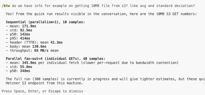
Read the numbers there carefully: sequential gives you 68 MB/s and a 142 ms p50. Parallel fan-out of 4 cuts per-request throughput in half — each individual fetch is now 348 ms p50 — but you finish four objects in roughly the time of one-and-a-half sequential ones. Fan-out is a latency trade, not a throughput trade. You spend bandwidth to compress p95.

The S3-numbers script does small, medium, and large object sizes at parallelism 1, 4, 8 — 300 samples per cell, ~1 hour total. Outputs a CSV plus a p50/p95/p99 table. Source: [TODO: link].

---

Recall as a function of nlist, nprobe

This is the result you’ll actually use to pick (nlist, nprobe) for production:

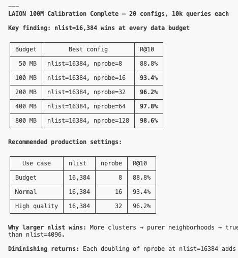
At LAION 100M, nlist=16,384 dominates at every byte budget. Bigger nlist → smaller, purer clusters → fewer wasted reads at the same nprobe. The trio of operating points worth memorising:

• Budget mode — 50 MB/query → 88.8% R@10. Use this if you’re cost-bound and your downstream can tolerate top-10 misses.
• Normal — 200 MB/query → 96.2% R@10. The “good defaults” point.
• High quality — 800 MB/query → 98.6% R@10. Use this if you’re recall-bound and the bandwidth is acceptable.

The diminishing returns are loud: 4× more bandwidth from 200→800 MB buys you ~2.4% more recall. Beyond 800 MB you’re well into territory where rerankers and query rewriting beat increasing nprobe.

---

The 400M cliff (and what’s next at 1B)

The trend at 10M → 100M is approximately linear: ~1% R@10 loss per 10× corpus growth at a fixed ~200 MB/query budget. At 400M, the same byte budget drops to 89.2% R@10 — a steeper fall than the trend predicts. The likely cause is nlist being below the ideal √N (~20,000 for 400M); a sweep at nlist=131,072 is the cheap next experiment.

---